Low-rank shift factors and electrical coordinates
2D embedding of electrical coordinates illustrates low-rank approximation of injection shift factors
Consider Figure 2 in this paper by Cuffe and Keane. The authors use injection shift factors to derive electrical distances. The electrical distance between nodes $i$ and $k$ is taken to be the sum of absolute values of all power flows induced in the network when 1 pu of active power is injected at $i$ and withdrawn at $k$. Having compiled all pairwise distances in a matrix, the authors then use multidimensional scaling to obtain 2D “electrical coordinates” for each bus. These coordinates may be plotted, and lines representing transmission lines may be added. The result is an electrically meaningful graph depiction of a power system.
Jon Martin (who was in my research group until he defended last year) noticed the sparsity of injection shift factors as he wrapped up his research. Pick a line in the network, and look at the sensitivity of its flow to injections at all buses. You will likely find that most sensitivities are tiny, but there are a couple with large magnitude. This suggests that the shift factor matrix is well-approximated by a low-rank matrix. To test this hypothesis, let’s combine SVD-based dimensionality reduction with the graph drawing procedure described in the previous paragraph, focusing on the IEEE 30-Bus system just like Cuffe and Keane did. Because the system has 30 nodes, the shift factor matrix $A$ has 30 singular value components. For $k\in[1,30]$, do the following:
- Let $U, S, V = \text{SVD}(A)$. A scatterplot of $\text{diag}(S)$ shows that a large portion of the sum of singular values is captured by the first 10 values:

- Compute a rank-$k$ approximation of $A$: $ A_k = U[:, 1:k]\cdot S[1:k, 1:k]\cdot V[:, 1:k]^\top $
- Derive a distance matrix $D_k$ from $A_k$ by summing the flows induced for a 1 pu injection and withdrawal at each pair of buses.
- Perform multidimensional scaling to obtain electrical coordinates $X_k$ for all nodes.
- Perform Procrustes analysis to align $X_k$ with $X_{k-1}$ (rotation is an extra degree of freedom in multidimensional scaling).
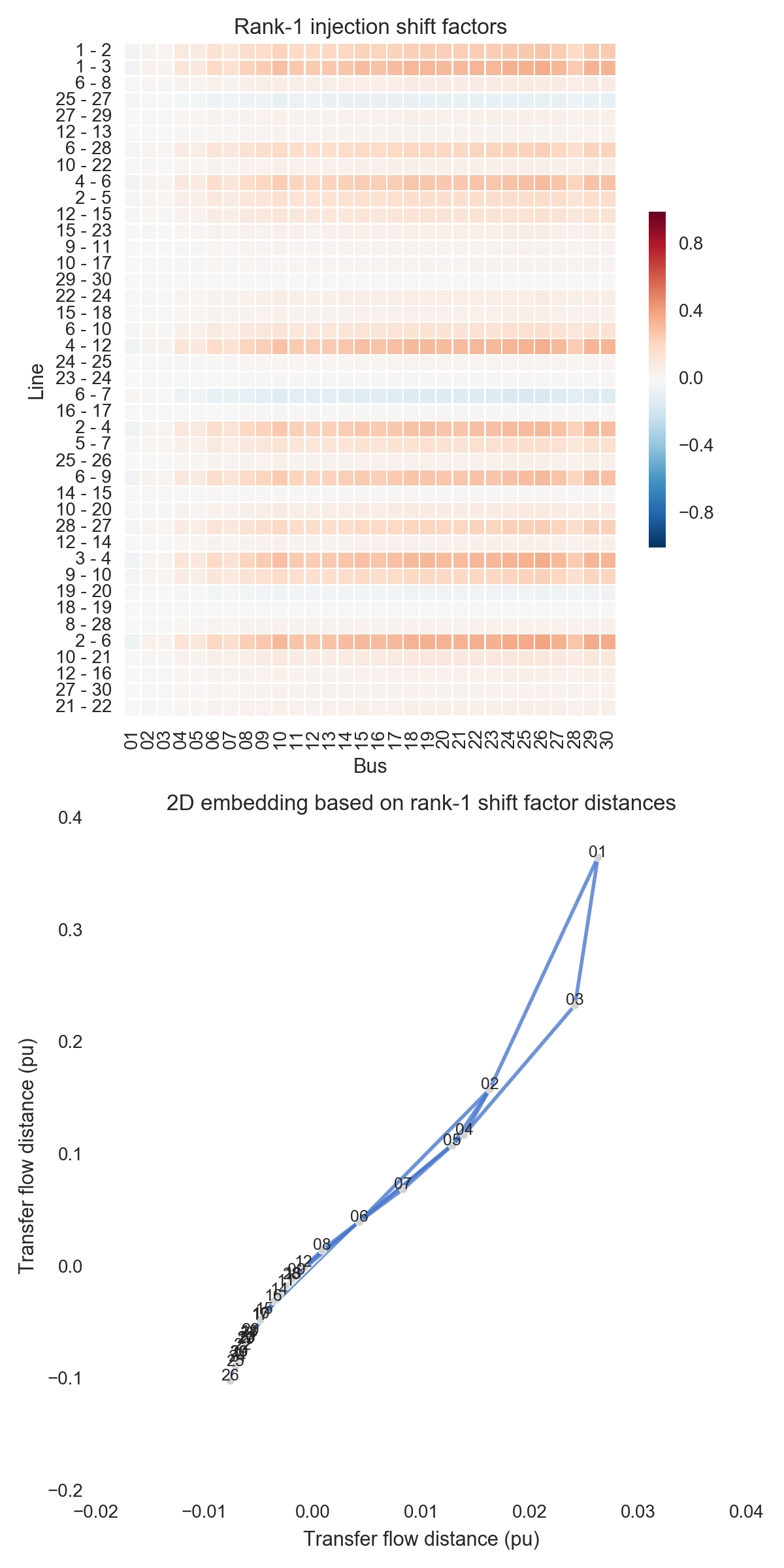
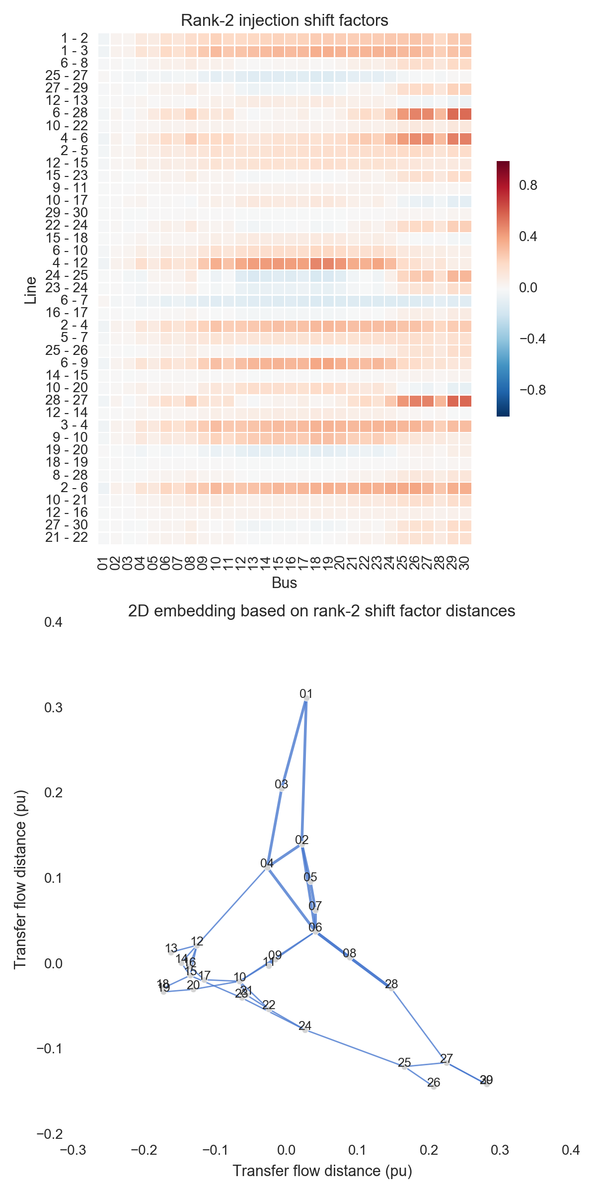
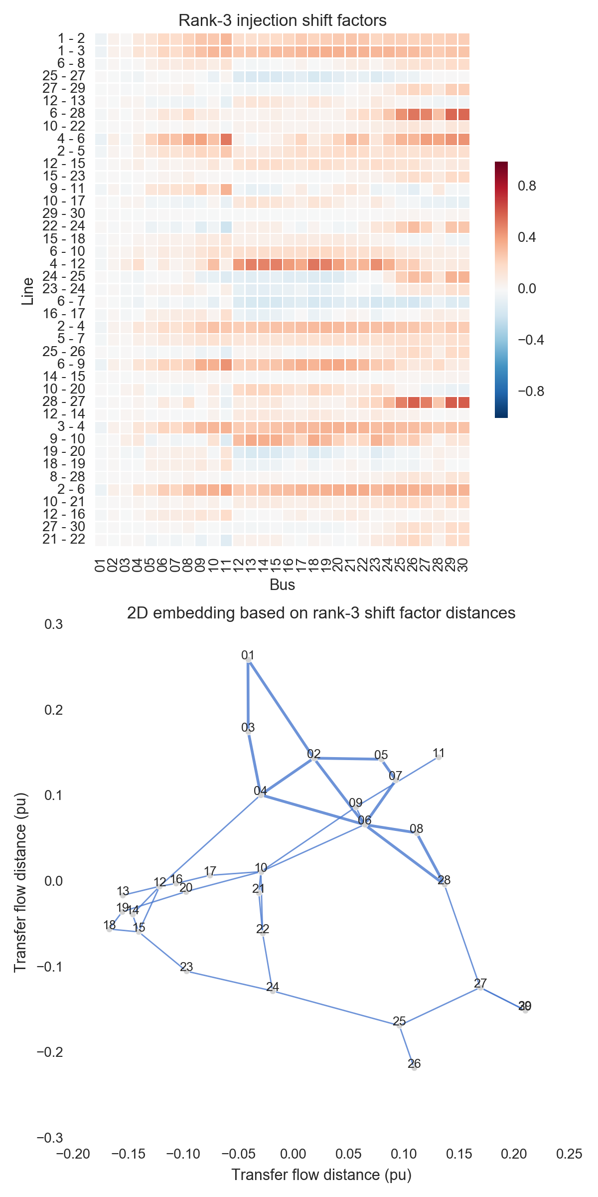
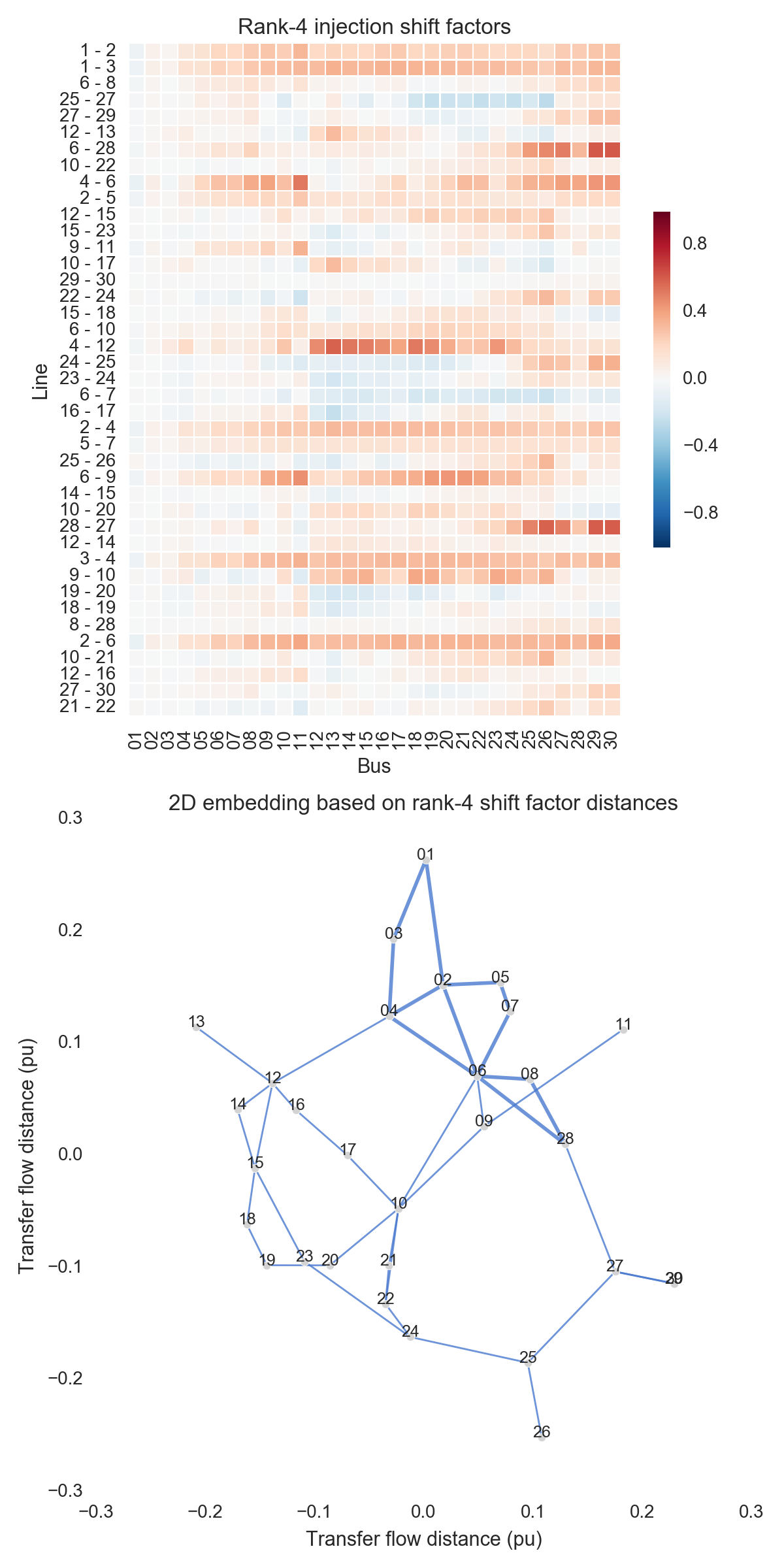
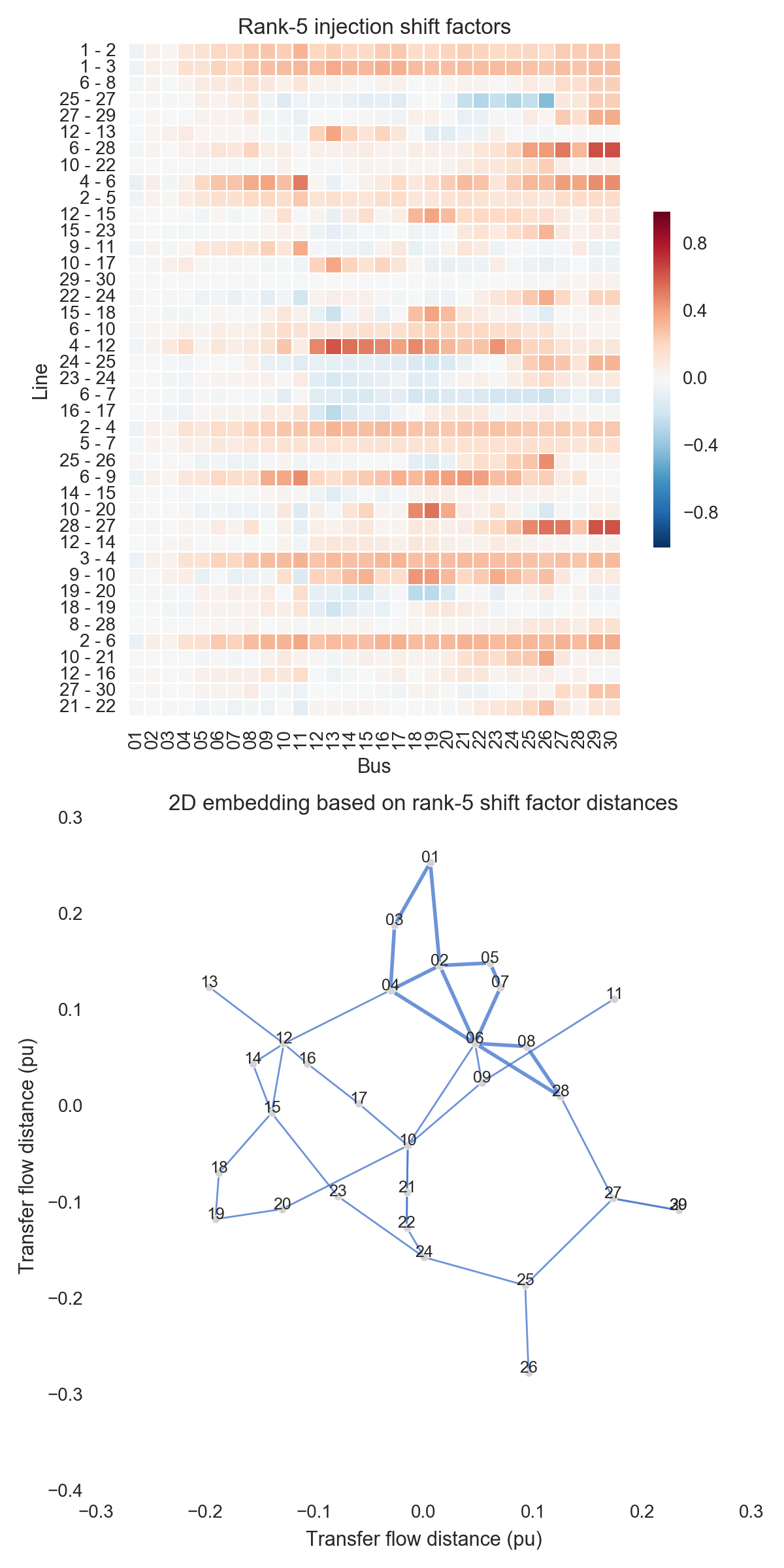
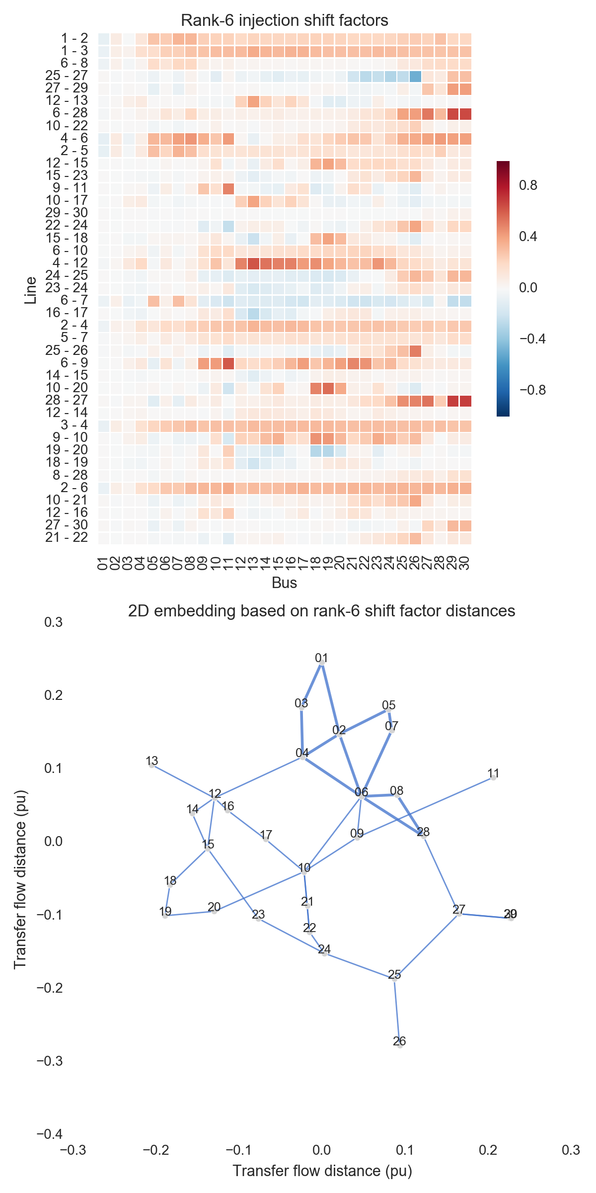
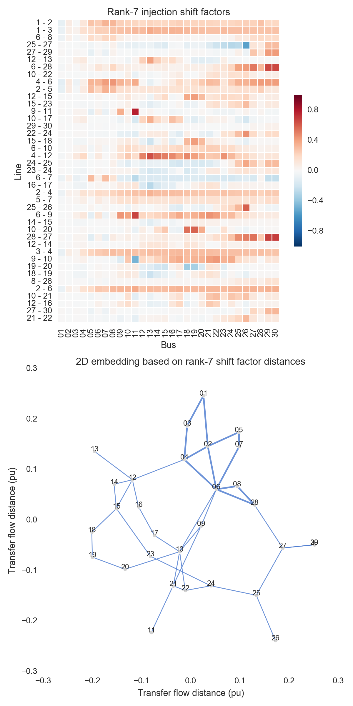
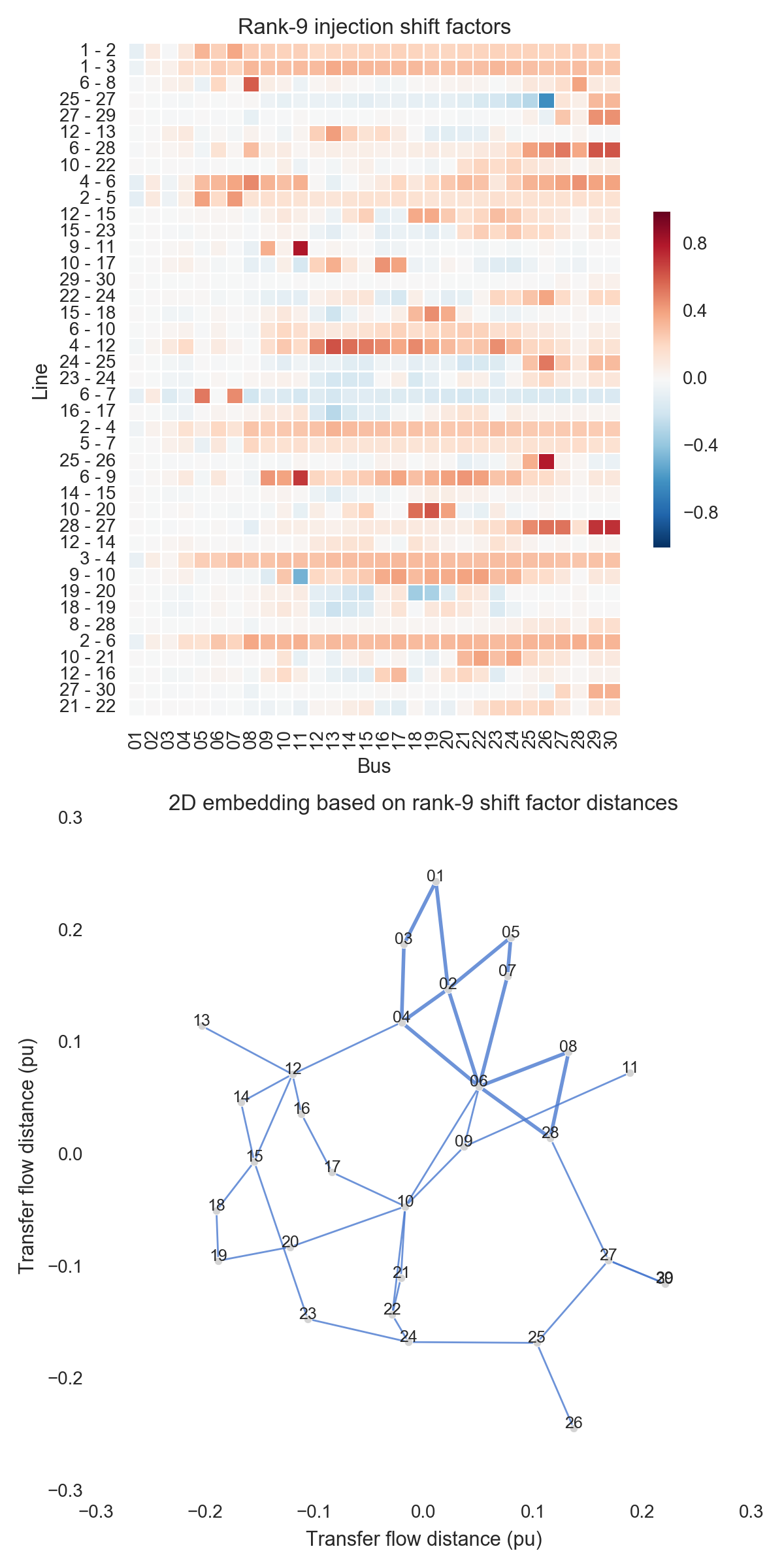
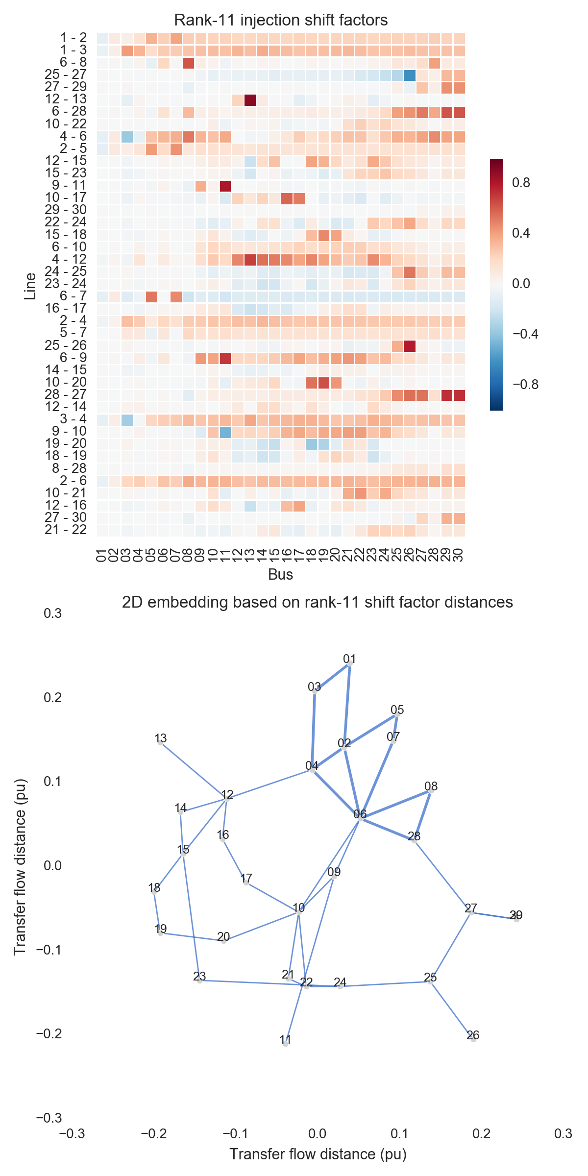
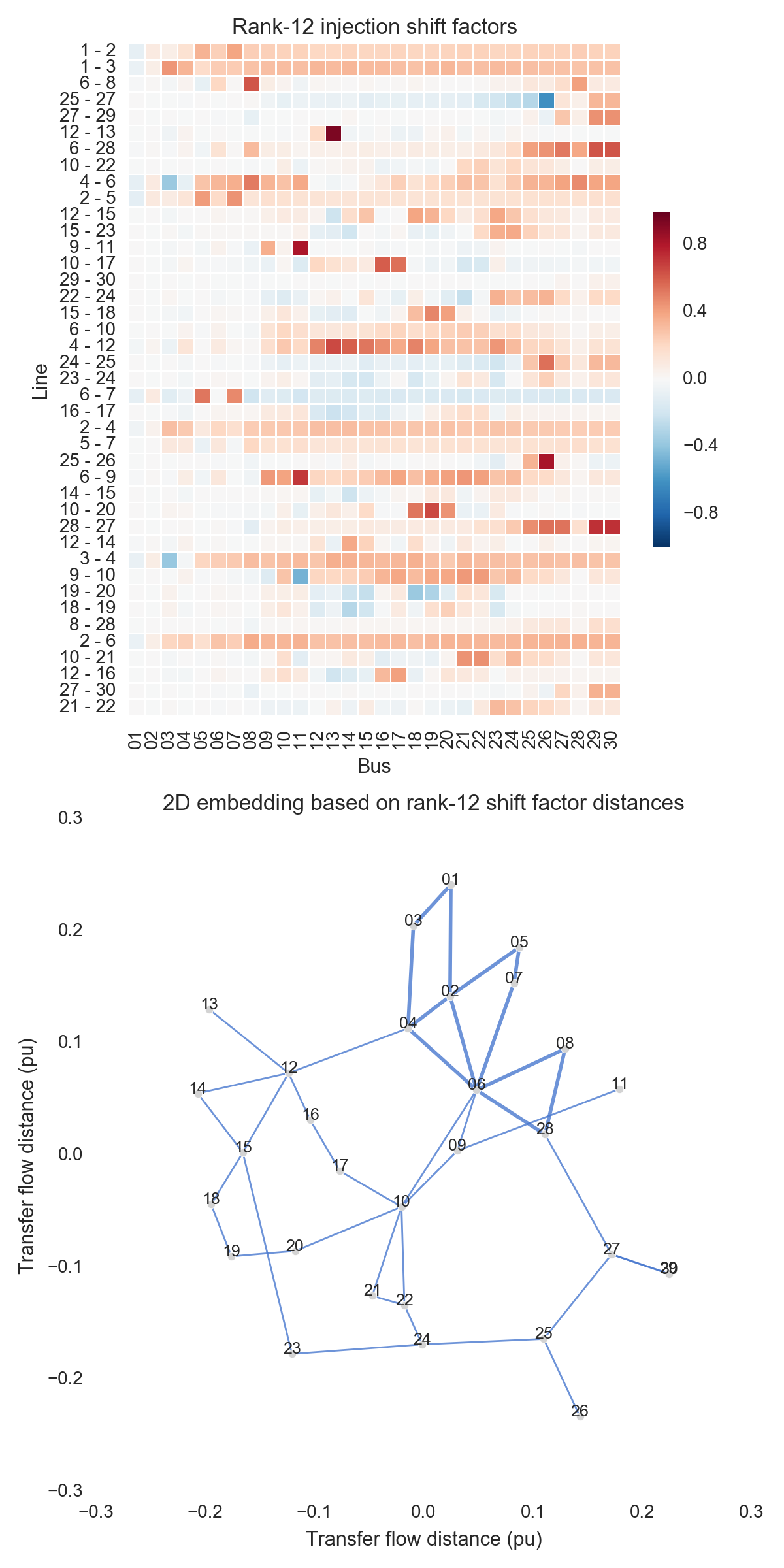
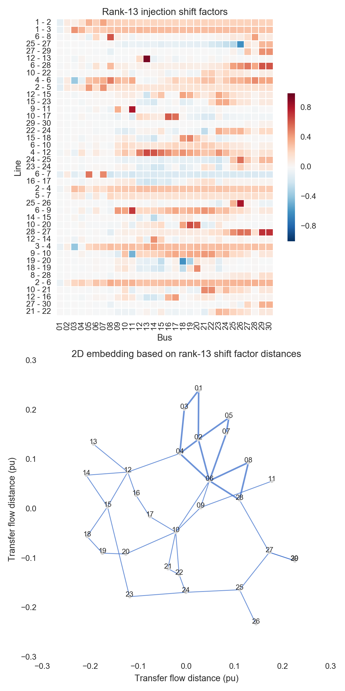
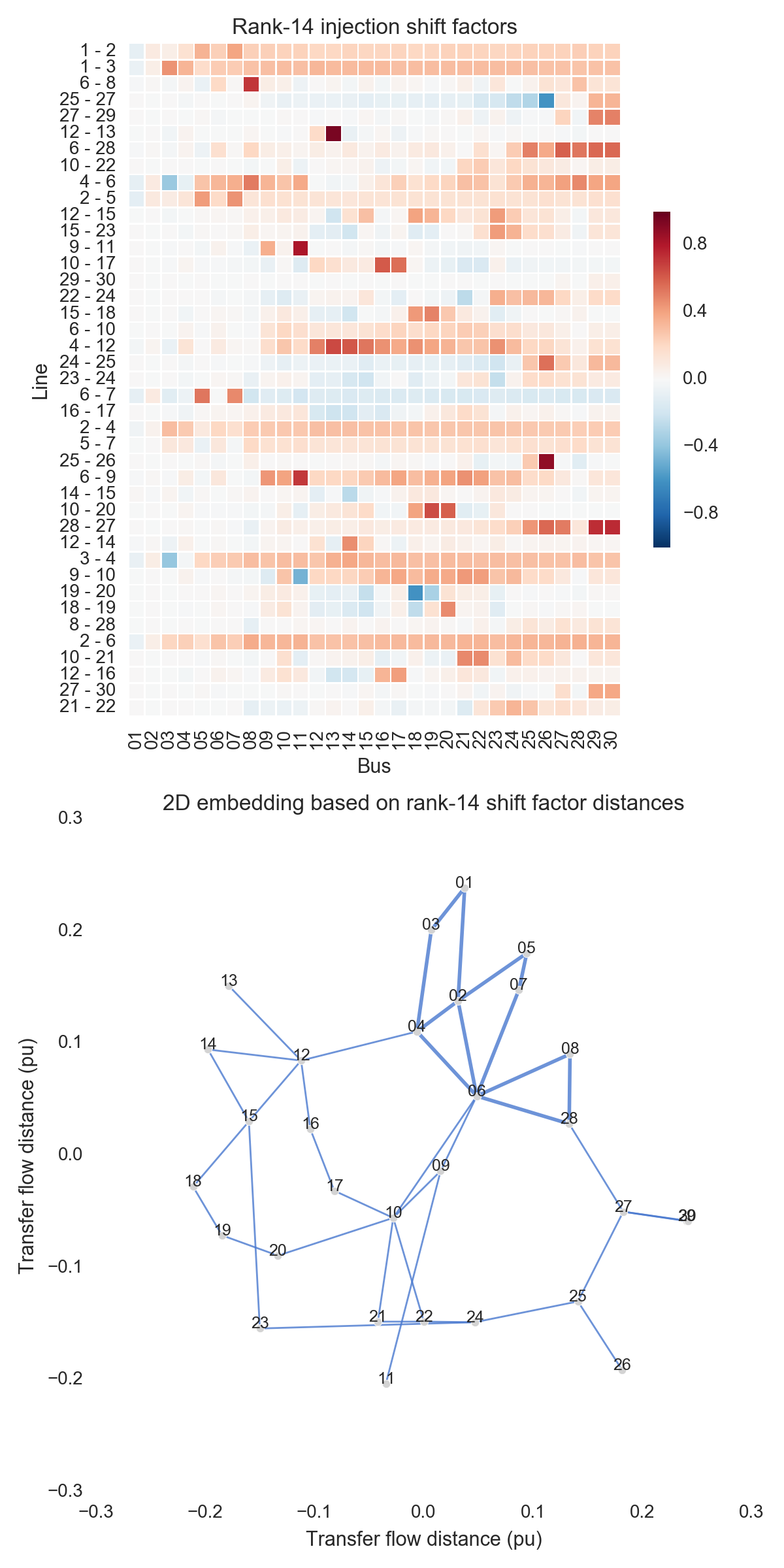
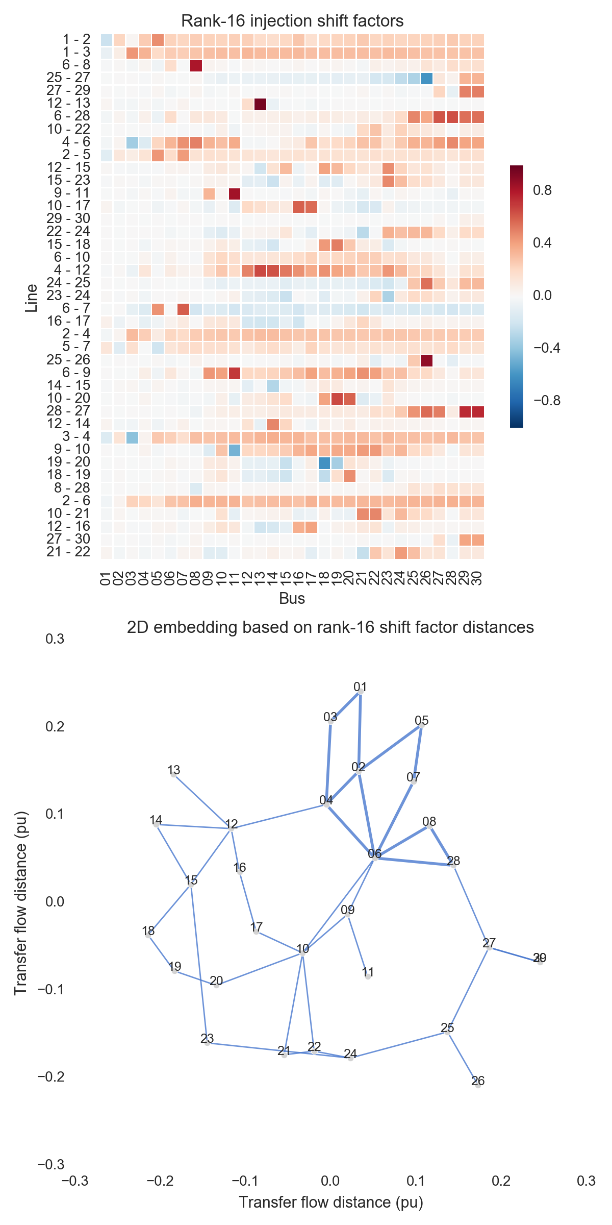
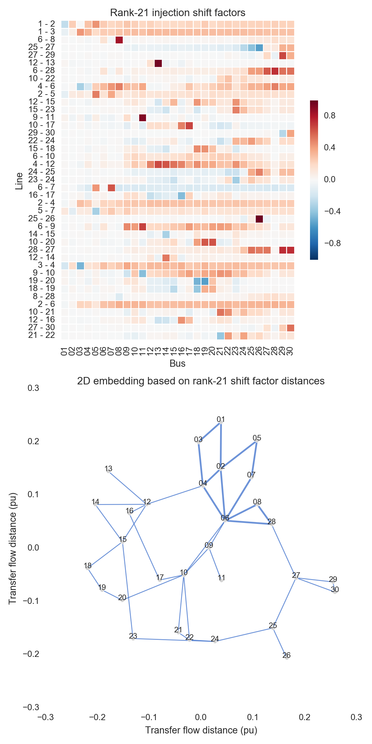
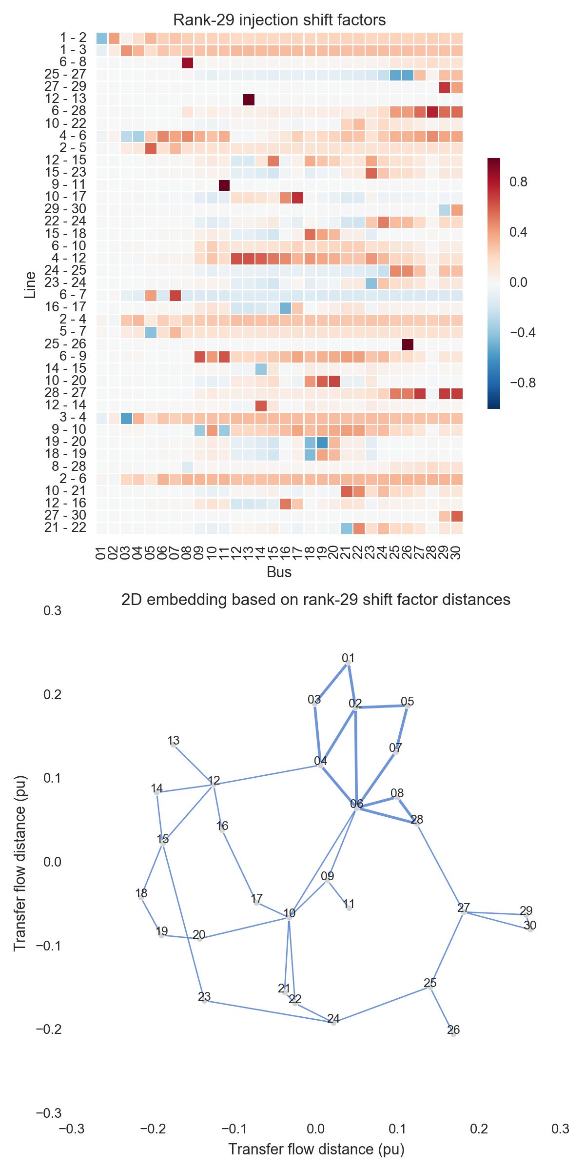
After performing the steps listed above, one can obtain the figures shown below. Use the buttons to flip through values of $k$. The top subfigure is a heatmap of $A_k$; at bottom is a graph visualization of $X_k$. Note that the high-voltage portion of IEEE 30 is designated by thicker lines.


A few observations:
- $X_1$ effectively places the nodes in a line; this is a 1D embedding of electrical distance. Note that the high-voltage portion of the grid (the “transmission backbone” already jumps out here).
- By the time we reach $X_5$, a great deal of the final structure is present.
- There is little qualitative difference between $X_{10}$ and $X_{29}$. Flipping between the two, we see that the last two features to be resolved are the separation between nodes 29 and 30 and the length of line $9-11$. Setting those relatively insignificant features aside, the graph possesses its final structure by $X_{10}$ (or even a little earlier).
- There is an intuitive explanation for shift factor sparsity: each line in the network is electrically close to just a few nodes. Most nodes are electrically distant, and are therefore unable to easily alter the line’s flow.
IEEE 30 is one of many commonly-used test networks. It may prove interesting to repeat this analysis for a collection of larger networks and look for trends.