Teaching

Integration of Renewable Energy (EECS 498)

I filled in twice as instructor for Dr. Hiskens’s power systems class in Winter 2017. The lectures introduced and summarized my research, but focused mostly on basics to ensure nobody was left behind (some of the students were new to the field).

Introduction to Control Systems (EECS 460)

Summary

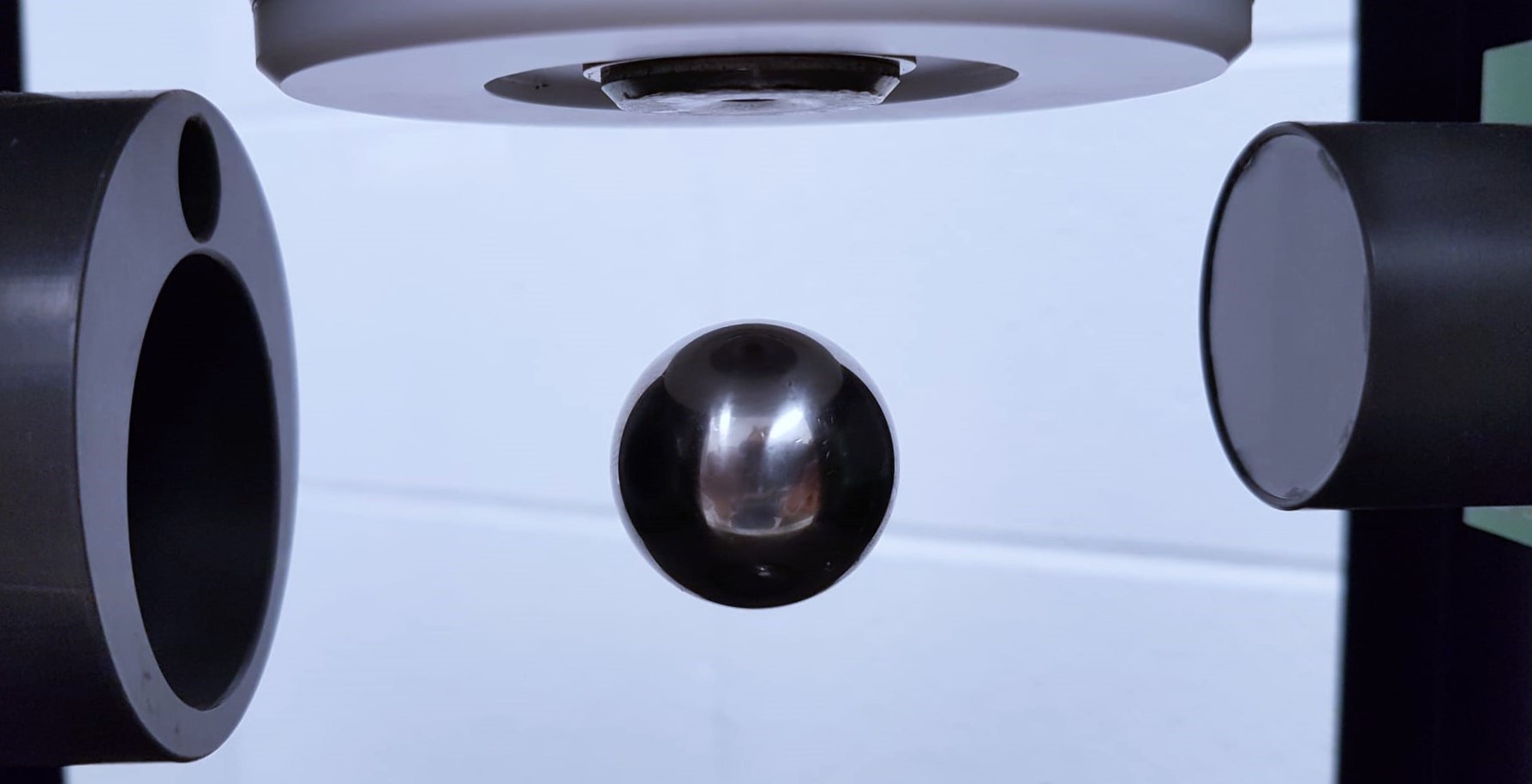
In Winter 2017 I was the Graduate Student Instructor for EECS 460, an introductory control systems class with roughly 80 students. My tasks included hosting twice-weekly discussion sessions, managing and editing homework documents, grading exams, and running the magnetic levitation lab (the final project).

Skills applied

Lecturing: I prepared a concise set of slides to summarize each week’s material and emphasize connections between topics as we progressed.
Active learning techniques: I was careful to give students time to work problems.
Visualization: I used Jupyter widgets to make an interactive visualization of a second-order transfer function response. This helped build intuitive understanding of the two parameters.
Gradescope: I scanned exam submissions and used Gradescope to set up online grading. This saved a great deal of time.
Scheduling: I used a Google Sheet to let students form into groups of 3-4 for the lab. I recorded a hyperlapse video to direct everyone to the obscure room. I oversaw each lab session, troubleshooting hardware and software problems as they came up. Finally, I used the University’s CTools site to collect and grade all reports.

Eigen-images (EECS 551)

Summary

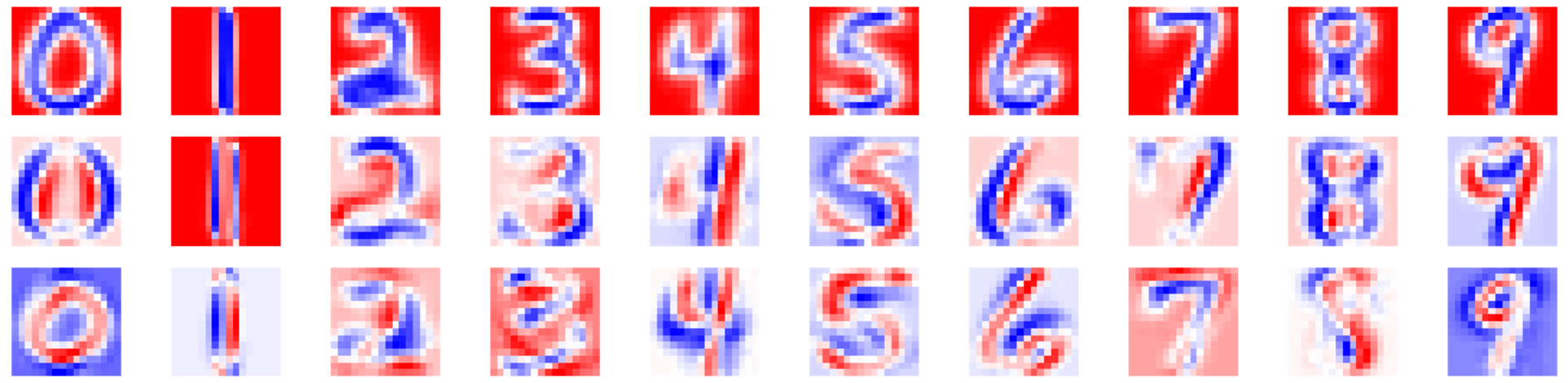
Professor Nadakuditi covers nearest-subspace classification in EECS 551. He uses a subset of the MNIST handwritten digit database to illustrate the concept. For each digit, a number of handwritten instances are grouped together, and the SVD is taken. The top $k$ components of this SVD characterize the digit’s subspace. Unlabeled test digits are then classified by determining its norm distance from each digit subspace. The nearest subspace determines the label. One powerful way to visualize what’s happening is to reason backwards: consider the top three SVD components of, say, the set of 0s in the training dataset. If we plot these components, we see that the first represents a sort of “mean 0”, the second represents a height adjustment, and the third represents width adjustment. Thus, a linear combination of these top three components yields a 0 with a particular thickness, height, and width.

The existing in-class demo consisted of static plots of the top three SVD components of the most interesting digits. Professor Nadakuditi would ask the class to interpret these plots, for example: what do plots of the top three components of the 2 database say about the way people write 2s? I made an interactive widget that allows students to choose any digit, then drag sliders to make a linear combination of that digit’s top three SVD components. The plot updates in real time, so students can immediately see the effects of adding or subtracting each component.

Skills applied

Layout: I wanted this demo to be as intuitive as possible, so the layout took some work. The final widget depicts the top three components with scalar weights underneath that update as the students drag sliders. The resulting linear combination is shown in a larger figure beneath the component figures.
Python
ipywidgets: this is the Python package that defines basic widget components like sliders and check-boxes.
matplotlib: to make the widget respond rapidly to student interaction, I had to be careful about figure redrawing. Partial redraws save computation time, allowing the widget to perform better.
Jupyter: the widget, other figures, and commentary live in an Jupyter notebook.

Background subtraction (EECS 551)

Summary

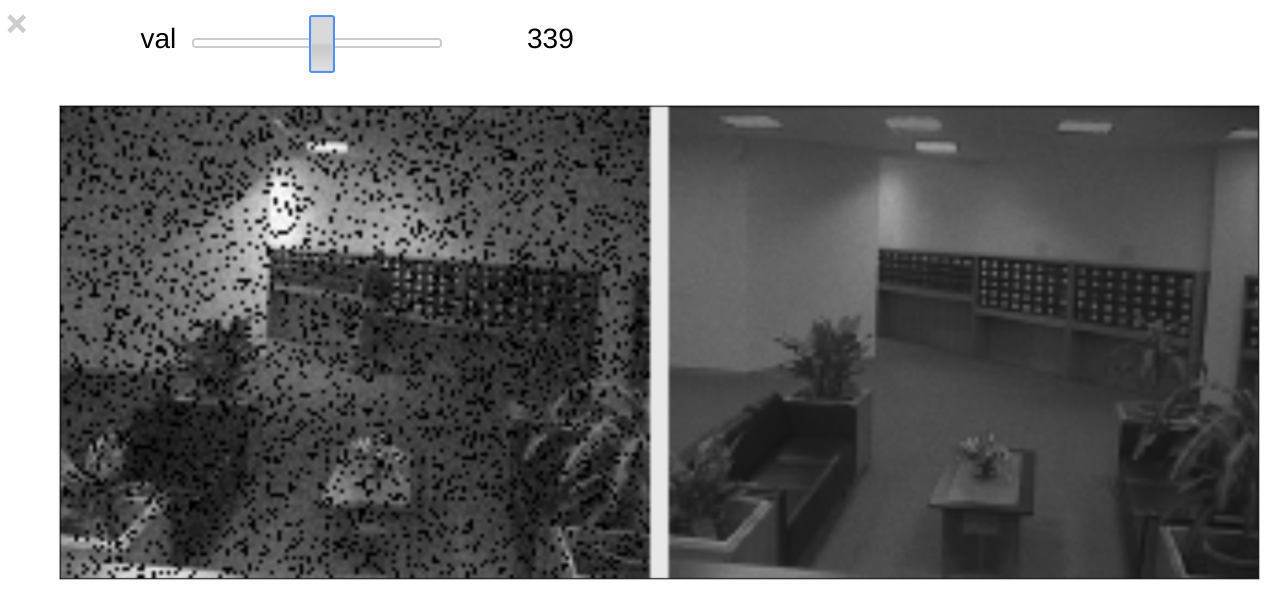
Professor Nadakuditi uses video background subtraction as a first illustration of SVD. First we view a black-and-white video as a three-axis matrix (X and Y for individual frames, Z for time). Then we reshape the video into a single matrix and take the SVD. When we reshape the first component back into video dimensions, we get the background of the scene. The remaining components contain all the motion in the video – the “high frequency” part, roughly speaking. This demo conveys the power of SVD in an intuitive way. SVD is able to cleanly isolate the background even when noise is added to the footage and some pixels are zeroed out. The demo encourages students to push SVD until it is no longer able to recover the background.

I translated the existing MATLAB demo into interactive Python and Julia notebooks.

Skills applied

MATLAB, Python, and Julia (and translation between them)
ipywidgets: this is the Python package that defines widget components like sliders. The notebooks I made contain use sliders to allow students to “scrub through” video footage.
matplotlib: the Python plotting package. Every time the slider is dragged, the figure must be updated. To minimize lag, I selectively redraw portions of the figure by referencing plot elements directly, rather than redrawing the entire canvas for every slider change.